Real analyses on real data. Each one was generated by the MCP Analytics team — interactive in the browser, exportable as PDF, citable, and reproducible. Click any card to open the full live report. Want to see one question answered at every depth, Snapshot through Capstone? See the examples.
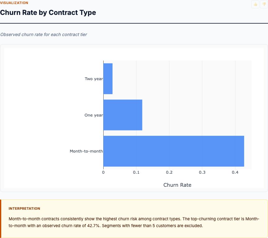
Logistic regression with feature importance, ranking the behavioral and demographic factors that predict whether a customer will churn.
View report →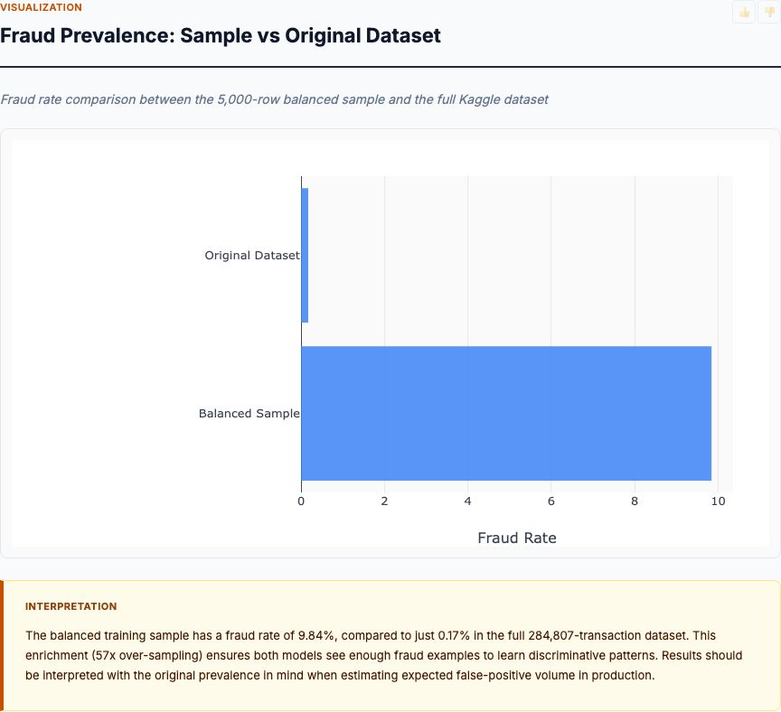
Isolation forest anomaly scoring on transaction features, surfacing the highest-risk outliers with explanation by feature contribution.
View report →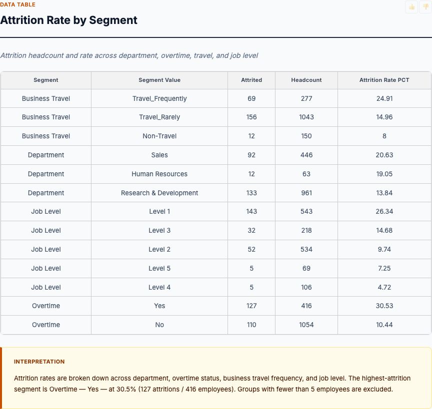
Logistic regression on attrition drivers — tenure, role, compensation, satisfaction — with odds ratios and a ranked driver list for retention planning.
View report →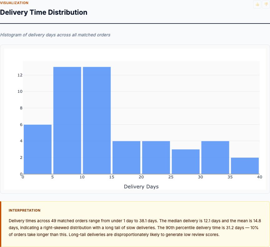
Regression analysis on order data identifying the delivery, timing, and fulfillment factors that most affect customer satisfaction scores.
View report →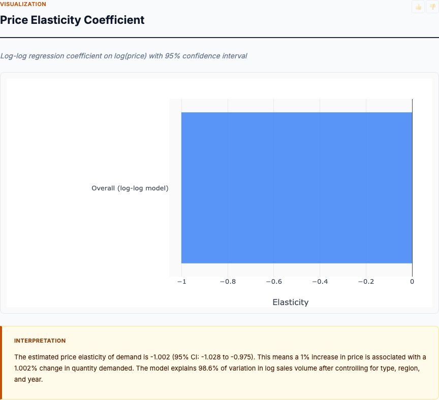
Price elasticity analysis on transaction data, estimating demand sensitivity by product category and identifying optimal pricing thresholds.
View report →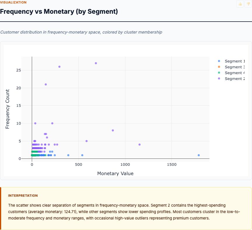
K-Means clustering on Recency, Frequency, Monetary value — bands customers into actionable retention and upsell segments with named profiles.
View report →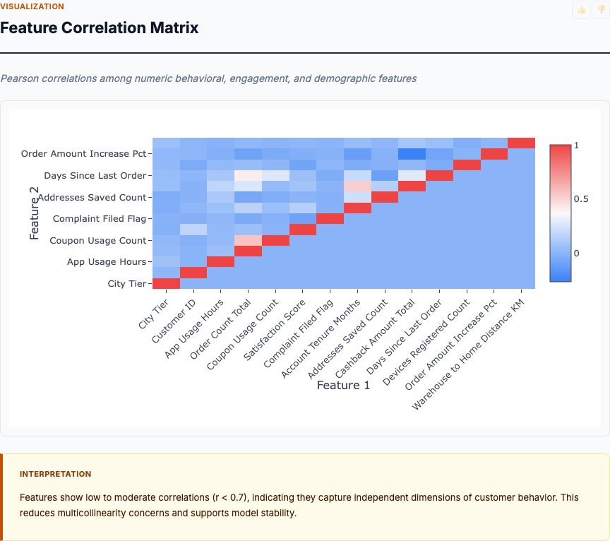
Random forest + logistic regression on behavioral and transactional features — outputs per-customer churn probability and ranked predictive drivers.
View report →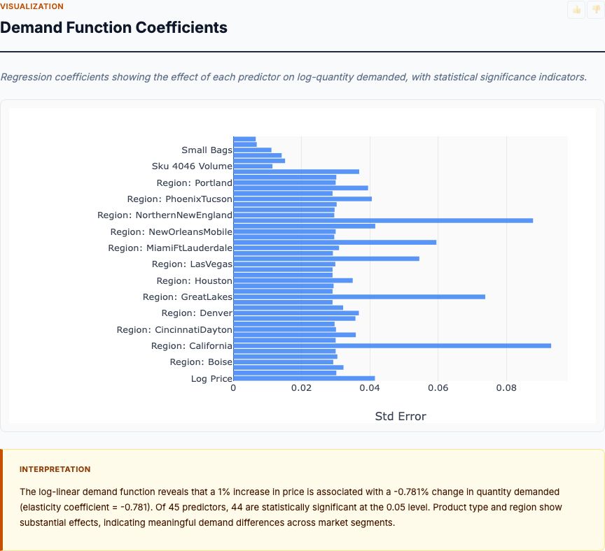
Log-log multiple regression on historical price and volume data — reports elasticity coefficients per category with confidence intervals.
View report →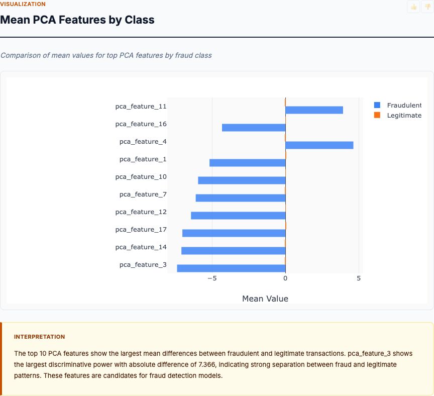
Statistical EDA across 28 PCA features plus amount and time — distributional comparisons, temporal heatmaps, and correlation matrices that surface the strongest fraud signals.
View report →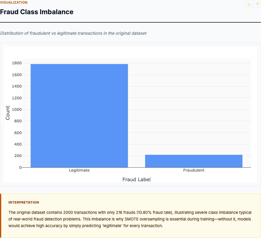
SMOTE-balanced training of logistic regression, random forest, and XGBoost — reports F1, AUC, precision, recall plus a ROC diagnostic and feature-importance ranking.
View report →
Seasonal decomposition plus ARIMA on monthly FMCG sales — produces point forecasts with prediction intervals and breaks out trend, seasonality, and residuals.
View report →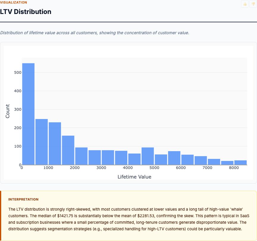
Distributional analysis of customer LTV with segment-by-contract breakdowns — surfaces high-value and at-risk cohorts and what subscription patterns drive each.
View report →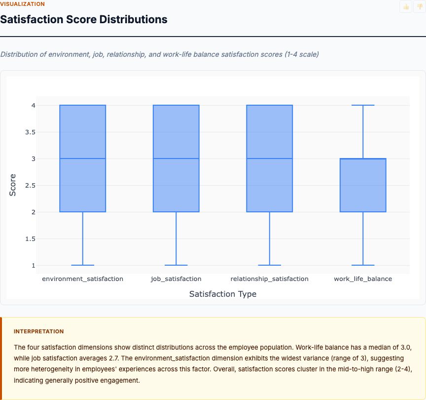
Exploratory analysis of IBM HR engagement and attrition data — satisfaction-by-department, tenure patterns, work-life balance, and how each dimension co-moves with attrition risk.
View report →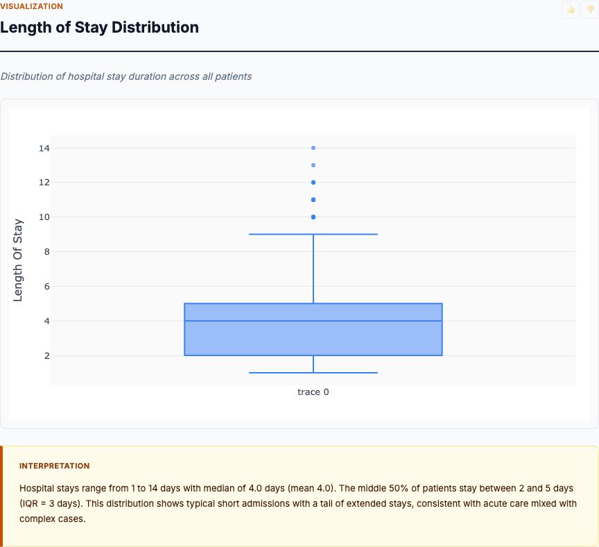
Multi-class classification on patient clinical features, comorbidities, labs and vitals — predicts length-of-stay bin and ranks the strongest predictors for care planning.
View report →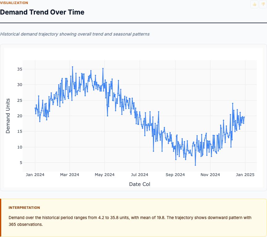
Time-series ARIMA forecasts per SKU/warehouse with seasonal components — informs reorder timing and inventory levels under varying supplier lead times.
View report →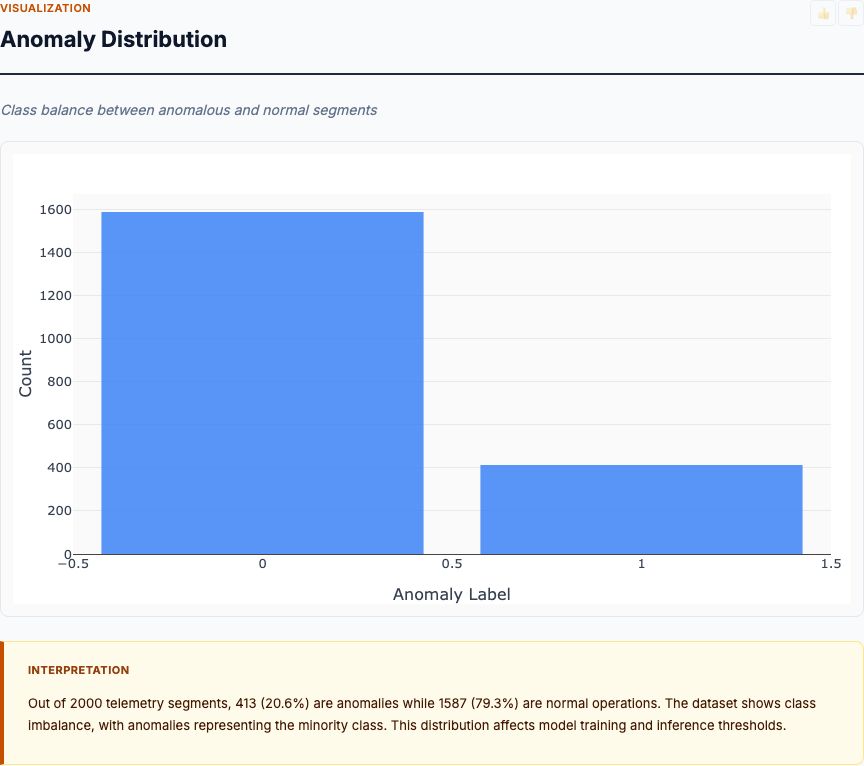
Supervised classification on signal statistical features — flags telemetry segments with anomalous behavior and explains them via feature contribution.
View report →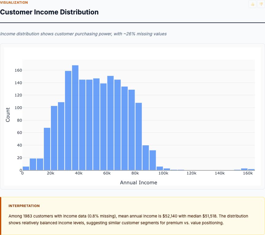
Personality and demographic profiling against spend across categories, purchase channels, and campaign response — produces actionable customer segments for client work.
View report →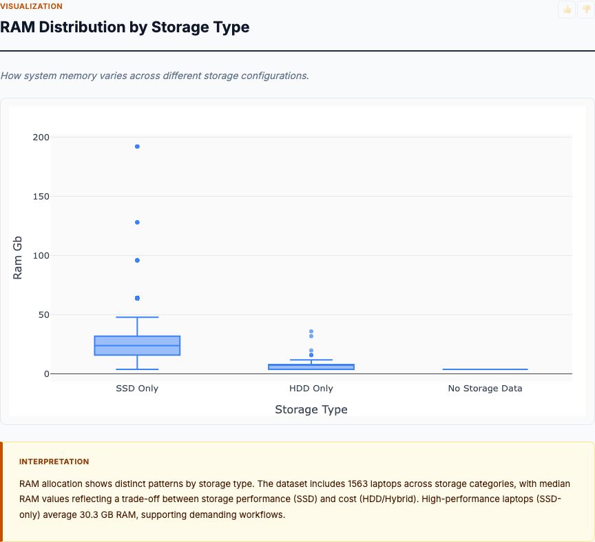
Automated profiling: distributions, correlations, missing-data audit, and a category-by-numeric overview that lands the analyst on the meaningful patterns in minutes.
View report →Every analysis includes the same components designed for real-world decision making.
Zoom, pan, and hover over charts. Residual plots, Q-Q plots, feature importance, time-series decompositions, and correlation matrices.
R², RMSE, MAE, p-values, confidence intervals, AIC/BIC — every relevant statistic for the analysis type. Nothing hidden.
Plain-English interpretation that explains what the numbers mean. Key findings, recommendations, and actionable next steps.
APA, MLA, Chicago, BibTeX in one click — paste straight into a paper, deck, or compliance filing. Methodology and source travel with the citation.
Validated R source code is embedded in every report. A skeptical reader can rerun it and get the same answer.
Fixed seeds, Docker isolation, validated R. Same input → same output on any machine, any day, forever.
Upload a CSV or connect a live source. Describe what you want to know. The team builds, validates, and ships the report.